Coloring cells in Google Spreadsheets may help to have a quick overview of numbers and figures. Like you can highlight all the decimal numbers in green. You don’t want to manually highlight each cell right? So, let spreadsheets do it for you.
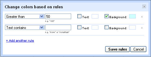
To apply conditional formatting, open up a blank spreadsheet document. Or just open up any of your previous spreadsheets. Lets take an example, say you have a spreadsheet with the prices of ten items. You want to highlight the items bought in quantities more than 5 and leave the rest intact. To do this, select all the columns containing numbers in your spreadsheet, i.e. the ones you want to apply conditional formatting to. They will appear in blue. Now, Right-click them and select “Change colors with rules”.

You can now choose options for setting color schemes of desired items. You can either modify the color of the text or the background of the cell. You can modify based on various constraints like Greater than, Less than, Text is Exactly, Text Contains, Date is etc. You can add more than one conditional formatting to a certain group of cells. Just click on “Add another rule” and you’ll be able to add more formatting rules.
You can select as many number of cells to apply formatting to. Anyway changing colors based on rules can be a very useful feature if used wisely.
